Can ML Detect Whipsaws?
I spent a couple of weeks training an XGBoost model to predict trade whipsaws, achieving excellent results on an 80/20 train/test split. However, when I tested the model on walk-forward data, it failed spectacularly: 92% performance drop from training to live testing. The model was memorising noise, not learning patterns. This post documents the journey from early optimism to the hard truth, and the valuable lessons I learned along the way.
An Experiment Worth Sharing
OK, so you got through the TL;DR and you're still here. You're probably thinking: What is a whipsaw?
This project started after I discovered how badly the Moving Average Convergence Divergence (MACD) indicator performs when the market moves sideways.
When MACD Meets Sideways Markets
Let's start by framing the problem. If you've ever traded using the MACD indicator, you know the pain. The MACD crossover is simple to implement and works beautifully... until it doesn't.
The issue isn't the MACD itself—it's what happens when markets move sideways. You get false breakouts. The MACD crosses bullish, triggering your entry signal, and then 1-3 bars later, the price pulls back. Your profit and loss (P&L) gets destroyed.
I experienced this firsthand with my SPIRIT trading bot. I was using the MACD cross to bullish during the build stage of the platform to keep things simple during debugging.
I like the MACD as a trigger—the logic is easy to implement and works well in trending markets. But this basic algorithm failed to make profit during testing.
The culprit? Whipsaw.
A "whipsaw" is when a technical indicator triggers an entry signal, only to immediately reverse direction. It's like getting whipped back and forth—hence the name.
Anatomy of a Whipsaw
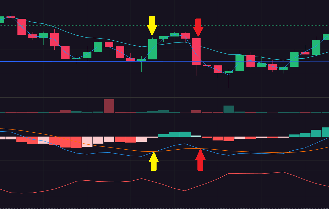
To truly understand a whipsaw, let's walk through a classic example using the MACD as the trigger. The sequence typically unfolds in four steps:
- The Signal: The MACD line crosses above its signal line. This is a classic bullish indicator, prompting traders to buy.
- The Bait: After the signal, the price moves up slightly. This initial confirmation makes the trade look promising, reinforcing the decision to enter.
- The Reversal: Just one to three price bars later, the market abruptly reverses and the price drops. This move is sharp enough to either trigger a stop-loss or put the position significantly "underwater."
- The Reality: The initial buy signal was deceptive, creating a classic false breakout. The market wasn't beginning a new uptrend; it was simply consolidating or moving sideways in a choppy market.
Unfortunately, this chips away at your capital through death by a thousand cuts. Your once-profitable MACD strategy now bleeds out.
The Idea: Can Machine Learning Spot the Fake Breakouts?
This is where the experiment began. I had a simple question: Can I train an XGBoost model to detect whipsaw trades before they happen?
The hypothesis was straightforward: Maybe the model could learn to spot when the market is cooling down and moving into consolidation. Maybe there are subtle patterns in the technical indicators at the point of the MACD cross that differentiate a real breakout from a false one.
It seemed like a reasonable idea. Machine learning is supposed to be good at finding non-linear patterns in data that humans miss, right?
So I set off to find out.
Version 1: Seeing the Future Really Helps ML (Nailed It!)
The first tests were encouraging. Actually, they were more than encouraging—they were exciting. I trained the XGBoost model on BTCUSD Q1 2025 data using a random 80/20 train/test split, and it showed good results.
But I've been here before. This isn't my first ML rodeo, and I had that feeling: "too good to be true."
The data showed 664 MACD cross triggers for the Q1 2025 dataset:
Training Metrics:
- ROC-AUC: 0.8097
- Precision: 97.25%
- Recall: 93.81%
- F1 Score: 0.9550
Validation Results:
- Profit Factor: 4.44 (vs 0.98 baseline)
- Win Rate: 68.18% (vs 31.93% baseline)
- Total P&L: +41.38% (vs -2.36% baseline)
The model caught 94% of whipsaws with 97% precision. Profit factor increased 4.5x. All the signs were pointing to "amazing." I was thinking this would catch a lot of bad trades, right? 🤔
The Red Flag I Missed
The model's top features were:
mfe_pct(46.1%) - Maximum Favorable Excursionmfe_bar_offset(22.4%) - Bars until MFEhistogram_value(12.5%) - MACD histogram
Here's the problem: MFE (Maximum Favorable Excursion) is only known after the trade completes. I was training the model on future indicators, then asking it to predict the past. Classic lookahead bias.
The excellent results weren't from learning market patterns—they were from data leakage. Nobody wants data leakage!
Version 2: Fixed the Leak (But Still Too Conservative)
After discovering the lookahead bias in v1, I immediately fixed it. Version 2 was my first "honest" model.
I fixed the lookahead bias by:
- ✅ Removing all post-trade features (MFE, MAE, bars_held)
- ✅ Using only pre-entry indicators (9 features available at cross time)
- ✅ Training on recent data only (3,500 trades from 2024 + Q1 2025)
V2 Performance:
- Win Rate: 37.2% (vs 32.4% baseline)
- Profit Factor: 1.27 (vs 0.96 baseline)
- ROC-AUC: 0.9314
- Blocks: 87.0% of trades (too conservative)
Key Discovery: ATR (volatility) emerged as the #1 predictor at 56% feature importance. This told me that high volatility MACD crosses have high whipsaw risk.
The Problem: While v2 was grounded in the present (no lookahead bias), it was too conservative. Blocking 87% of trades meant missing too many opportunities. The win rate improved slightly, but the model was being overly cautious.
Status: Honest but limited - it needed more data and better generalisation.
Version 3: The "Proper" Model
Looking at v2's overly conservative behaviour, I decided to train on much more data, more data = more good! So my thought process was: train the model on diverse market conditions spanning multiple bull/bear cycles. This should improve generalisation, right?
I expanded the dataset by:
- ✅ Using 11 years of data (2013-2025-03, 27,959 trades)
- ✅ Covering multiple market regimes (Mt. Gox crash 2014, COVID bull run 2020-2021, FTX crash 2022, etc.)
- ✅ Keeping only pre-entry features (no lookahead bias)
Tests started to show that the model was catching over 70% of the whipsaw trades. That's fantastic! Now, it wasn't detecting ALL bad trades—just the whipsaw trades, which is exactly what I designed it to do. I wanted to keep the model focused on picking up those specific 1-3 bar false breakouts, not trying to predict every losing trade.
Training Metrics (11 years of BTCUSD data):
- ROC-AUC: 0.7823
- Precision: 95.6% (95.6% of predictions are correct!)
- Recall: 77.3% (catches 77% of whipsaws!)
- F1 Score: 0.8544
Below is a binary classifier: Good Trade vs Whipsaw (bad trade I want to avoid).
Confusion Matrix (Test Set):
                     Predicted
                 Good      Whipsaw
Actual Good      315       183
       Whipsaw   1158      3936
Translation:
- True Positives: 3,936 whipsaws correctly blocked
- False Positives: 183 good trades incorrectly blocked (only 4.4%!)
- False Negatives: 1,158 whipsaws missed (22.7%)
- True Negatives: 315 good trades correctly allowed
Now I needed to create a baseline to see the improvement for V3. Let's run a test with just the MACD (no ML filter) and then the same data with the V3 filter.
Trading Performance Impact:
Both baseline and V3 were tested on the same historical dataset (2013-2025-03, 31,371 trades):
Baseline (No Filter):
- Total P&L: -542.79%
- Win rate: 32.52%
- Profit factor: 0.94
V3 ML-Filtered:
- Total P&L: +644.96%
- Win rate: 38.31%
- Profit factor: 1.17
- P&L improvement: +218.8%
Bam! The model works! It's blocking 73.6% of trades but improves P&L by 218%. Feature importance shifted to price_vs_sma200 (27.8%), suggesting the model learned that trend positioning matters across different market cycles.
OK, I think I have done it, a working ML filter, but the TradeBot had other ideas!
Now let's take a moment to discuss the disappointing win rates. 38% win rate! I was disappointed with this result. I thought 55-65% win rates would be what I was looking for.
A Reality Check: Why 38% Win Rate is Actually Good
When I first saw the V3 model results, I was disappointed. A 38% win rate? I'd been expecting something much higher. Surely a machine learning model trained on 11 years of data should win more often than it loses, right?
Wrong.
Let me explain why this thinking was flawed—and why 38% is actually excellent performance.
Win Rate Doesn't Equal Profitability
Here's the counterintuitive truth about trading: you can be profitable with a 30% win rate, or lose money with a 70% win rate. What matters isn't how often you win—it's how much you make when you win versus how much you lose when you lose.
Consider two traders:
Trader A:
- Win rate: 70%
- Average win: +$100
- Average loss: -$300
- Net result after 100 trades: -$2,000 loss
Trader B:
- Win rate: 35%
- Average win: +$500
- Average loss: -$100
- Net result after 100 trades: +$11,000 profit
Trader B wins only 35% of the time but makes 5x more money because winners are bigger than losers.
The Metrics That Actually Matter
In trading, profit factor is the gold standard:
Profit Factor = Total Gains / Total Losses
- PF < 1.0 = Losing strategy (you're bleeding money)
- PF = 1.0 = Breakeven (wasting your time)
- PF > 1.0 = Profitable strategy (making money)
- PF > 2.0 = Excellent strategy (rare!)
The baseline MACD strategy had a profit factor of 0.94—meaning for every dollar gained, we lost $1.06. We were slowly going broke with a 32.52% win rate.
The V3 ML-filtered model achieved a profit factor of 1.17—for every dollar lost, we made $1.17. The strategy turned consistently profitable despite only winning 38% of the time.
Why 38% is Actually Excellent
Let's put this in context:
| Strategy | Win Rate | Profit Factor | Total P&L (11 years) | Verdict |
|---|---|---|---|---|
| Baseline MACD | 32.52% | 0.94 | -542.79% | Losing money |
| ML-Filtered | 38.31% | 1.17 | +644.96% | Making money |
| Improvement | +5.79% | +24.7% | +1,187.75% | Night and day |
A 5.79% improvement in win rate translated to:
- Turning a -542.79% loss into a +644.96% gain
- A 1,187% P&L swing
- Crossing from unprofitable to profitable
That's the power of even small win rate improvements when combined with proper risk management.
The MACD crossover strategy is a trend-following system. It loses often in a sideways market (whipsaws) but wins big when a real trend emerges. A 38% win rate is right in the sweet spot for this type of strategy.
The Real Problem Wasn't Win Rate
Looking at the baseline results, the real problem was:
- Whipsaw rate: 61.52% (most trades failed quickly)
- Profit factor: 0.94 (losing overall)
- Average P&L: -0.02% (death by a thousand cuts)
The ML model improved these by:
- Blocking 73.6% of trades (highly selective)
- Reducing whipsaw rate to 55.71% (-5.81%)
- Boosting profit factor to 1.17 (crossed profitability threshold)
The lesson: Don't focus on win rate alone. Focus on profit factor and total P&L. A 38% win rate with positive expectancy beats a 60% win rate with negative expectancy every single time.
Oh OK, so the idea I had is working! V3 is filtering out the whipsaw death by a thousand cuts. I now better understand the win rate and P&L—it's starting to make sense.
I've validated my hypothesis that started this project, right?
Spoiler Alert
As you'll see in the next section, these impressive metrics were based on test set validation—not true out-of-sample performance. When I tested the model on genuinely unseen Q2 2025 data, the model exploded in a ball of flames. Well, not quite, but precision collapsed to 6% (from 95.6% on historical test).
The model never saw data from AFTER the training period. My 'test set' was 20% of historical data, not true future data.
But the lesson about win rates still stands: profitability ≠ win rate. (Yeah Tim, try and find something positive from this rollercoaster of ML computing.)
Put Your Money Where Your ML Is
So I'm feeling pretty good. I've systematically built up and tested the model. I've tested and validated the model's performance and documented all the steps. Now picture me in a white lab coat with a clipboard!
I've taken a logical approach to this idea, and next I'll test the model on current candle data.
I have my trading account ready with my hard-earned cash!
And my prediction is that I'll see similar results to the backtest.
Wrong.
The model's performance got worse. What worked on the generalized 11 years of data—bull markets, bear markets, low volatility periods, high volatility periods—all have different "whipsaw fingerprints."
On Q2 2025 data (April-June 2025, my unseen test set), the model wasn't performing well at all. Precision collapsed to 6% (from 95.6% on historical test). The model was blocking 91.8% of trades (vs 73.6% on training data), being far too conservative when faced with new market conditions.
Head in my hands, I just couldn't understand it! Tell me how... no, why... no, ahhhhh.
OK, crushed dreams... But let's think about this. How can the model be so bad?
Well, it turns out that bad data makes bad days.
I.T. Fire
Ring ring, ring ring. "Hello, this is IT support, how can I help?"
Unfortunately, I don't have an IT help desk I can call. No, I built the "enterprise home network" that is running the TradeBot, and it was at this point the Proxmox server said... "No more."
Critical Incident: SQL01 VM Data Disk Failure
What Happened:
- Morning: Attempted to run Q1 2025 model validation to investigate the Q2 2025 failure
- Discovery: PostgreSQL I/O errors blocked all database queries
- Root Cause: 2TB USB SSD (SSD01_2T) hardware failure - SQL01 VM data disk inaccessible
- Impact: 50GB database with 210 Million rows at risk, all ML validation work blocked
Emergency Response Timeline:
09:00 - Attempted Q1 2025 validation → PostgreSQL I/O errors
10:00 - Diagnosed 2TB USB SSD (SSD01_2T) hardware failure
11:00 - Emergency migration: SQL01 data disk from 2TB to 500GB backup drive
13:00 - USB power cycle restored 2TB drive to service (health unknown)
14:00 - VM 107 boot failure: fstab configuration mismatch with new disk
17:00 - Day ended with VM offline, comprehensive documentation completed
Impact:
- Zero code progress on November 7th (full day consumed by crisis response)
- All ML validation work blocked (no database access)
- The corrupt data invalidated my Q2 2025 tests. I had to rerun everything.
So what have I learned from this? That a Dell USFF desktop acting as a server can't handle 210 million rows of data! Who would have guessed? 🤦
The issue took me 3 days to diagnose and resolve. It was corrupt data at the heart of the model's poor performance initially. Bad data!
I'm not going to go into detail on how I fixed the home network. I think that's a story all of its own.
However, you can rest assured that I now have a couple of cloud-based servers running in a datacenter with dedicated hardware. No more data corruption, failed model training, dropped SSH sessions, or unresponsive hosts.
Well, I hope. :)
Back Online!
With new infrastructure ready, built and tested, I uploaded the 50GB of OHLC training data to a new PostgreSQL server and started reindexing the 210 million rows of data.
Let's get back to testing the model. Does it work?
Not quite. After fixing the data corruption issues, I started to see that the larger dataset gave lower performance. The model seemed to be "too generalised." The idea of more data = more good was not correct.
This was an interesting data point for me, as I found that a 3-6 month dataset seemed to be a good balance for the model.
I retrained a new model on Q1 2025 data (3 months), and the results looked better than the 11-year v3 model, but still not great. The new model achieved 14.3% precision on Q2 validation (better than v3's 6%, but still far from production-ready).
Retraining: Reality Check
So the large dataset was a non-starter. OK, well let's see if we can retrain the model more often to "adjust to" new market conditions. Let's say, train the model on 3 months of data and then retrain each week to add the most up-to-date data to the model.
Let's use a walk-forward test on the model. This test is the gold standard in trading system development. It simulates real-world conditions:
- Train on 90 days of data
- Test on the next week
- Retrain weekly with updated data
- Compare to a static model trained once
Test Period: 1 January - 1 March, 2025 (9 weeks, 57 trades)
Auto-Retrain Triggers:
- F1 score < 0.3, or
- Miss rate > 80%
The Results Were Brutal
Week-by-Week Pattern:
| Week | Training F1 | Testing F1 | Outcome |
|---|---|---|---|
| 1 | 0.974 | 0.000 | ⚠️ RETRAIN |
| 2 | 0.976 | 0.000 | ⚠️ RETRAIN |
| 3 | 0.950 | 0.000 | ⚠️ RETRAIN |
| 4 | 0.900 | 0.000 | ⚠️ RETRAIN |
| 5 | 0.919 | 0.000 | ⚠️ RETRAIN |
| 6 | 0.889 | 0.400 | ✅ First success! |
| 7 | 0.889 | 0.000 | ⚠️ RETRAIN |
| 8 | (retrained) | 0.500 | ⚠️ Static model better |
| 9 | 0.970 | 0.000 | ⚠️ RETRAIN |
Retrain Frequency: 8 out of 9 weeks (89%)
Final Comparison:
- Rolling Retrain F1: 0.074
- Static Model F1: 0.087
- Performance Drop: 92% (training to testing)
The Pattern Was Clear
Every single time I retrained:
- Model achieves F1 = 0.90-0.97 on training data ✅
- Model achieves F1 = 0.00-0.07 on testing data ❌
- Triggers retrain
- Repeat
The model was memorising noise patterns from the training window that didn't exist in the next week's data. Frequent retraining didn't fix overfitting—it made it worse by constantly fitting to more noise.
What Went Wrong?
At this point on the TradeBot rollercoaster, I was feeling broken! The amazing results at the start of the project to the brutal failure at the end just didn't add up for me.
I had missed something, and I needed to know why.
After a day of reviewing this project, I believe it's a mixture of backtesting issues and allowing the model to mark its own homework.
Yes, I think I had inadvertently allowed the model to see the "test" data, and this was how it was able to seem like it was smashing it out of the park!
When it used unseen data, it just fell over. The model was simply memorising patterns, not learning at all.
End Result for ML
The final conclusion is: Whipsaw is not detectable with ML using entry-point technical indicators. The information needed (news, liquidity, orderbook) isn't in the data.
It seems that there are no "indicators" that the model can use to predict if a whipsaw will happen.
What I Learned from This Rollercoaster
A lot! Whipsaws are fundamentally unpredictable.
Whipsaws are caused by:
- Sudden news events
- Liquidity gaps
- Stop-loss cascades
- Market maker games
- Random noise
None of these things show up in technical indicators at the point of entry. By the time the MACD crosses, the information you need to predict a whipsaw isn't in the data yet.
The big takeaway is: when something looks too good, it usually is.
In the future when training ML models, I need to make sure of the following:
1. Backtest Properly with Temporal Splits
What I did wrong: Used random 80/20 split on time-series data
Why it's wrong: Random splits on time-series data cause temporal leakage - training data from 2023 can "see" test data from 2015
How to fix it:
# ❌ Wrong: Random split
train, test = train_test_split(df, test_size=0.2, random_state=42)

# ✅ Correct: Temporal split
# The first 80% of the time period for training, the last 20% for testing.
# This ensures test data comes AFTER training data chronologically.
split_date = '2024-09-01'
train = df[df['date'] < split_date]
test = df[df['date'] >= split_date]
2. Backtesting is Fast but Not Predictive
Backtesting is a fast way to get results for model performance but not the best for predicting real performance. You need to test on TRUE future data that comes after your training period ended.
3. Keep Training Data Separate from Walk-Forward Data
Once you use the data, it's done! You can't use this data for testing the model at a later date. Keep good data hygiene (it's tempting to use the latest dataset).
4. Document Everything
So you can find your way back if you go down the wrong turn.
Red Flags I Should Have Caught
Looking back, here were the warning signs:
-
Train F1 = 0.95, Test F1 = 0.85 - Good scores, but on the SAME time period
- ⚠️ Should have tested on LATER data (e.g., Apr-Jun 2025)
-
95.6% precision - Suspiciously perfect
- ⚠️ Real-world ML rarely achieves >90% on noisy financial data
-
Model blocks 73.6% of trades - Very aggressive
- ⚠️ High precision often means overfitting
-
Feature importance shifted between v2 and v3
- v2: ATR 56% (recent data)
- v3: SMA200 27.8% (11 years)
- ⚠️ Both models may be overfitting to their respective periods
If I'd caught these, I would have demanded true out-of-sample testing before celebrating.
This is the first time I've gone back through the process to document my work. It has forced me to focus and review each step. I can see that I jumped around with training datasets and rushed ahead without fully understanding the results. Early good results spurred me on to make bigger steps: more data, more technical indicators, more training, and so on.
However, this has been a great experience, and I now feel like I understand why this failed. With any luck, it will help build the next model.